HPF detector, orders, and fibers
The HPF detector is a 2048x2048 pixel 1.7 micron cutoff H2RG detector, controlled by a SIDECAR ASIC and a SAM interface board. Data are obtained using 4 readout amplifiers (channels), in the up-the-ramp mode. Channels run vertically on the detector (e.g. Ch1: 512:1023,0:2047; Ch2: 0:511,0:2047; etc.). The detector has 2040 x 2040 active pixels surrounded a 4 pixel wide band of non-light-sensitive reference pixels. Reference pixels are retained in all 2d images.
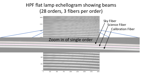
There are 3 separate spectra that fall on the detector from 3 separate fibers as follows:
| Fiber | Description |
|---|---|
| Sky fiber | Fiber on the sky offset from the science fiber for taking a spectrum of the sky emission. The spectrum from this fiber can be used to subtract sky lines from the science spectrum. |
| Science fiber | Fiber placed on the science target by the HET. Contains the spectrum of the science target. |
| Calibration fiber | Fiber connected to the HPF calibration bench. Normally it contains the spectrum of the laser frequency comb for simultaneous wavelength calibration with each science spectrum for precision-RV measurements. For low S/N or non-precision-RV targets, the comb is generally turned off. |
The light from a single echelle order for a single fiber is called a “beam.” The HPF echellogram consists of 28 orders repeated for each of the 3 fibers for a total of 84 beams.
Where the data are stored
The HPF data are stored at the Texas Advanced Computing Center (TACC, https://www.tacc.utexas.edu) and accessed in a similar fashion to other HET instruments. For information on creating accounts and logging into TACC see: https://hydra.as.utexas.edu/?a=help&h=56
Data are organized by “date” and “observation number”. Dates are the UT date of the observation in the format YYYYMMDD. Each ramp (exposure) has its own four digit observation number (OBSNUM). Observation numbers start at 1 for the first ramp in a night, and simply increment upwards for each following ramp.
All the HPF data are stored in the following directory on TACC:
/work/03946/hetdex/maverick/YYYYMMDD/hpf/raw/OBSNUM/
/work/03946/hetdex/maverick/YYYYMMDD/hpf/reduced/OBSNUM/
./raw/ directories contain the unprocessed up-the-ramp fits files
./reduced/ directories contain processed slope images and extracted, wavelength calibrated spectra
The nightly manifests
Manifests are electronically generated observing logs that list all ramps taken for each night. They are formatted in fixed-width format columns. Each night’s manifest is separated by noon local time at HET so that all the calibrations (evening and morning) are listed with the associated science data. Note that the evening calibrations mostly have UT dates from the day before the science data is taken. Manifests are useful for identifying the ObsNum corresponding to you data, as well as identifying calibration frames that you may want.
The manifests are all stored in the named as hpf_YYYYMMDD.list in the base hpf directory for each night (e.g. /work/03946/hetdex/maverick/YYYYMMDD/hpf/).
Example manifest for UT Date of 20180526:
             UT-Timestamp    UT-Date   ObsNum                            Frame   ObsType      iTime         QProg             Object
  2018-05-25T21:28:33.952   20180525     0040   Slope-20180525T212805_R01.fits       Sci      213.0                    LFC_CalibTest
  2018-05-25T22:28:58.484   20180525     0041   Slope-20180525T222831_R01.fits       Cal      319.5                             Dark
  2018-05-25T22:39:05.903   20180525     0042   Slope-20180525T223838_R01.fits       Cal       85.2                 Alpha Bright Cal
  2018-05-25T22:41:13.814   20180525     0043   Slope-20180525T224046_R01.fits       Cal       85.2                 Alpha Bright Cal
  2018-05-25T22:43:21.892   20180525     0044   Slope-20180525T224254_R01.fits       Cal       85.2                 Alpha Bright Cal
  2018-05-25T22:45:29.766   20180525     0045   Slope-20180525T224502_R01.fits       Cal       85.2                 Alpha Bright Cal
  2018-05-25T22:47:37.495   20180525     0046   Slope-20180525T224709_R01.fits       Cal       85.2                 Alpha Bright Cal
  2018-05-25T22:49:45.580   20180525     0047   Slope-20180525T224917_R01.fits       Cal       85.2                 Alpha Bright Cal
  2018-05-25T22:51:53.505   20180525     0048   Slope-20180525T225124_R01.fits       Cal       85.2                 Alpha Bright Cal
  2018-05-25T22:54:01.507   20180525     0049   Slope-20180525T225338_R01.fits       Cal       85.2                 Alpha Bright Cal
  2018-05-25T22:56:09.252   20180525     0050   Slope-20180525T225545_R01.fits       Cal       85.2                 Alpha Bright Cal
  2018-05-25T23:21:01.701   20180525     0051   Slope-20180525T232031_R01.fits       Sci      468.6                 Alpha Bright FCU
  2018-05-25T23:31:20.194   20180525     0052   Slope-20180525T233050_R01.fits       Cal     479.25                 Alpha Bright FCU
  2018-05-25T23:40:02.488   20180525     0053   Slope-20180525T233938_R01.fits       Cal     479.25                 Alpha Bright FCU
  2018-05-25T23:48:44.854   20180525     0054   Slope-20180525T234819_R01.fits       Cal     479.25                 Alpha Bright FCU
  2018-05-25T23:58:31.178   20180525     0055   Slope-20180525T235803_R01.fits       Cal      106.5                          LFC FCU
  2018-05-26T00:01:00.323   20180526     0001   Slope-20180526T000036_R01.fits       Cal      106.5                          LFC FCU
  2018-05-26T00:03:29.646   20180526     0002   Slope-20180526T000303_R01.fits       Cal      106.5                          LFC FCU
  2018-05-26T00:05:58.857   20180526     0003   Slope-20180526T000530_R01.fits       Cal      106.5                          LFC FCU
  2018-05-26T00:08:28.198   20180526     0004   Slope-20180526T000803_R01.fits       Cal      106.5                          LFC FCU
  2018-05-26T00:10:57.402   20180526     0005   Slope-20180526T001030_R01.fits       Cal      106.5                          LFC FCU
  2018-05-26T00:14:09.278   20180526     0006   Slope-20180526T001339_R01.fits       Cal     159.75                          LFC Cal
  2018-05-26T00:17:31.793   20180526     0007   Slope-20180526T001703_R01.fits       Cal     159.75                          LFC Cal
  2018-05-26T00:20:54.258   20180526     0008   Slope-20180526T002027_R01.fits       Cal     159.75                          LFC Cal
  2018-05-26T00:24:16.815   20180526     0009   Slope-20180526T002351_R01.fits       Cal     159.75                          LFC Cal
  2018-05-26T00:27:39.522   20180526     0010   Slope-20180526T002716_R01.fits       Cal     159.75                          LFC Cal
  2018-05-26T00:31:02.089   20180526     0011   Slope-20180526T003034_R01.fits       Cal     159.75                          LFC Cal
  2018-05-26T00:34:45.949   20180526     0012   Slope-20180526T003417_R01.fits       Cal     159.75                       Etalon Cal
  2018-05-26T00:38:08.473   20180526     0013   Slope-20180526T003742_R01.fits       Cal     159.75                       Etalon Cal
  2018-05-26T00:41:31.052   20180526     0014   Slope-20180526T004106_R01.fits       Cal     159.75                       Etalon Cal
  2018-05-26T02:28:07.032   20180526     0015   Slope-20180526T022738_R01.fits       Cal      958.5                    UNe Slave Cal
  2018-05-26T02:44:49.105   20180526     0016   Slope-20180526T024422_R01.fits       Cal      958.5                    UNe Slave Cal
  2018-05-26T03:01:31.231   20180526     0017   Slope-20180526T030106_R01.fits       Cal      958.5    UT18-2-005      UNe Slave Cal
  2018-05-26T03:57:07.794   20180526     0018   Slope-20180526T035637_R01.fits       Sci     330.15                           HR4131
  2018-05-26T04:04:03.586   20180526     0019   Slope-20180526T040334_R01.fits       Sci      319.5                       HR4131_lfc
  2018-05-26T04:34:05.163   20180526     0020   Slope-20180526T043337_R01.fits       Sci      511.2   PSU18-2-004             CM_Dra
  2018-05-26T04:50:25.938   20180526     0021   Slope-20180526T044955_R01.fits       Sci     308.85   ENG18-2-003             GJ_436
  2018-05-26T04:56:17.727   20180526     0022   Slope-20180526T045548_R01.fits       Sci     308.85   ENG18-2-003             GJ_436
  2018-05-26T05:02:09.516   20180526     0023   Slope-20180526T050141_R01.fits       Sci     308.85   ENG18-2-003             GJ_436
  2018-05-26T05:21:52.723   20180526     0024   Slope-20180526T052123_R01.fits       Sci     308.85   PSU18-2-004    PM_J17464+2743W
  2018-05-26T06:43:36.440   20180526     0025   Slope-20180526T064306_R01.fits       Sci     308.85   ENG18-2-003             GJ_699
  2018-05-26T06:49:28.199   20180526     0026   Slope-20180526T064859_R01.fits       Sci     308.85   ENG18-2-003             GJ_699
  2018-05-26T06:55:19.928   20180526     0027   Slope-20180526T065452_R01.fits       Sci     308.85   ENG18-2-003             GJ_699
  2018-05-26T07:01:11.850   20180526     0028   Slope-20180526T070044_R01.fits       Sci     308.85   ENG18-2-003             GJ_699
  2018-05-26T07:07:03.530   20180526     0029   Slope-20180526T070637_R01.fits       Sci     308.85   ENG18-2-003             GJ_699
  2018-05-26T07:20:12.524   20180526     0030   Slope-20180526T071944_R01.fits       Sci     330.15   PSU18-2-003           G_227-22
  2018-05-26T07:26:25.564   20180526     0031   Slope-20180526T072602_R01.fits       Sci      319.5   PSU18-2-003           G_227-22
  2018-05-26T07:32:28.013   20180526     0032   Slope-20180526T073200_R01.fits       Sci     330.15   PSU18-2-003           G_227-22
  2018-05-26T07:45:26.172   20180526     0033   Slope-20180526T074459_R01.fits       Sci     159.75   PSU18-2-004           G_227-22
  2018-05-26T07:54:40.652   20180526     0034   Slope-20180526T075412_R01.fits       Sci     308.85   PSU18-2-004            GJ_725B
  2018-05-26T08:07:38.675   20180526     0035   Slope-20180526T080709_R01.fits       Sci     330.15   PSU18-2-008              KELT9
  2018-05-26T08:18:29.045   20180526     0036   Slope-20180526T081759_R01.fits       Sci      724.2   PSU18-2-004     PM_J16148+6038
  2018-05-26T08:31:16.581   20180526     0037   Slope-20180526T083052_R01.fits       Sci   713.5500   PSU18-2-004     PM_J16148+6038
  2018-05-26T09:24:45.295   20180526     0038   Slope-20180526T092415_R01.fits       Sci      468.6   PSU18-2-004     PM_J16139+3346
  2018-05-26T10:16:27.459   20180526     0039   Slope-20180526T101557_R01.fits       Sci      681.6   PSU18-2-004        PSU18-2-004
  2018-05-26T10:28:32.388   20180526     0040   Slope-20180526T102807_R01.fits       Sci      681.6   PSU18-2-004        PSU18-2-004
  2018-05-26T10:53:24.722   20180526     0041   Slope-20180526T105255_R01.fits       Cal      319.5                             Dark
  2018-05-26T11:00:20.516   20180526     0042   Slope-20180526T105951_R01.fits       Cal      106.5                          LFC FCU
  2018-05-26T11:02:49.832   20180526     0043   Slope-20180526T110225_R01.fits       Cal      106.5                          LFC FCU
  2018-05-26T11:05:18.955   20180526     0044   Slope-20180526T110452_R01.fits       Cal      106.5                          LFC FCU
  2018-05-26T11:07:48.214   20180526     0045   Slope-20180526T110719_R01.fits       Cal      106.5                          LFC FCU
  2018-05-26T11:10:17.496   20180526     0046   Slope-20180526T110952_R01.fits       Cal      106.5                          LFC FCU
  2018-05-26T11:12:46.755   20180526     0047   Slope-20180526T111219_R01.fits       Cal      106.5                          LFC FCU
  2018-05-26T11:15:47.934   20180526     0048   Slope-20180526T111520_R01.fits       Cal      106.5                          LFC Cal
  2018-05-26T11:18:17.259   20180526     0049   Slope-20180526T111753_R01.fits       Cal      106.5                          LFC Cal
  2018-05-26T11:20:46.592   20180526     0050   Slope-20180526T112020_R01.fits       Cal      106.5                          LFC Cal
  2018-05-26T11:23:15.772   20180526     0051   Slope-20180526T112247_R01.fits       Cal      106.5                          LFC Cal
  2018-05-26T11:25:44.819   20180526     0052   Slope-20180526T112520_R01.fits       Cal      106.5                          LFC Cal
  2018-05-26T11:28:14.159   20180526     0053   Slope-20180526T112747_R01.fits       Cal      106.5                          LFC Cal
  2018-05-26T11:30:43.511   20180526     0054   Slope-20180526T113015_R01.fits       Cal      106.5                          LFC Cal
  2018-05-26T11:33:12.790   20180526     0055   Slope-20180526T113248_R01.fits       Cal      106.5                          LFC Cal
  2018-05-26T11:35:41.949   20180526     0056   Slope-20180526T113515_R01.fits       Cal      106.5                          LFC Cal
  2018-05-26T11:38:53.883   20180526     0057   Slope-20180526T113825_R01.fits       Cal     202.35                 Alpha Bright FCU
  2018-05-26T11:42:59.096   20180526     0058   Slope-20180526T114234_R01.fits       Cal      213.0                 Alpha Bright FCU
  2018-05-26T11:47:57.526   20180526     0059   Slope-20180526T114731_R01.fits       Cal       85.2                 Alpha Bright Cal
  2018-05-26T11:50:05.474   20180526     0060   Slope-20180526T114938_R01.fits       Cal       85.2                 Alpha Bright Cal
  2018-05-26T11:52:13.443   20180526     0061   Slope-20180526T115146_R01.fits       Cal       85.2                 Alpha Bright Cal
  2018-05-26T11:54:21.405   20180526     0062   Slope-20180526T115354_R01.fits       Cal       85.2                 Alpha Bright Cal
  2018-05-26T11:56:29.333   20180526     0063   Slope-20180526T115602_R01.fits       Cal       85.2                 Alpha Bright Cal
  2018-05-26T11:58:37.275   20180526     0064   Slope-20180526T115810_R01.fits       Cal       85.2                 Alpha Bright Cal
  2018-05-26T12:00:45.149   20180526     0065   Slope-20180526T120018_R01.fits       Cal       85.2                 Alpha Bright Cal
  2018-05-26T12:02:53.122   20180526     0066   Slope-20180526T120226_R01.fits       Cal       85.2                 Alpha Bright Cal
  2018-05-26T12:05:01.079   20180526     0067   Slope-20180526T120434_R01.fits       Cal       85.2                 Alpha Bright Cal
  2018-05-26T12:07:40.995   20180526     0068   Slope-20180526T120712_R01.fits       Cal      106.5                          LFC Cal
  2018-05-26T12:10:10.231   20180526     0069   Slope-20180526T120946_R01.fits       Cal      106.5                          LFC Cal
  2018-05-26T12:12:39.464   20180526     0070   Slope-20180526T121213_R01.fits       Cal      106.5                          LFC Cal
  2018-05-26T12:17:48.564   20180526     0071   Slope-20180526T121721_R01.fits       Cal     159.75                       Etalon Cal
  2018-05-26T12:21:11.233   20180526     0072   Slope-20180526T122044_R01.fits       Cal     159.75                       Etalon Cal
  2018-05-26T12:24:33.659   20180526     0073   Slope-20180526T122408_R01.fits       Cal     159.75                       Etalon Cal
  2018-05-26T12:27:56.319   20180526     0074   Slope-20180526T122733_R01.fits       Cal     159.75                       Etalon Cal
  2018-05-26T12:31:40.286   20180526     0075   Slope-20180526T123110_R01.fits       Cal      958.5                    UNe Slave Cal
  2018-05-26T12:48:22.235   20180526     0076   Slope-20180526T124755_R01.fits       Cal      958.5                    UNe Slave Cal
  2018-05-26T13:05:04.257   20180526     0077   Slope-20180526T130439_R01.fits       Cal      937.2                    UNe Slave Cal
Fixed-width columns of the manifests:
| Column Number | Character range | Column Name | Description |
|---|---|---|---|
| 1 | 3-26 | UT-Timestamp | Universal time a ramp was taken in format YYYY-MM-DDTHH:MM:SS.SSS |
| 2 | 27-37 | UT-Date | UT Date ramp was taken in format YYYYMMDD |
| 3 | 38-46 | ObsNum | Observation number for the ramp |
| 4 | 47-89 | Frame | Name of frame that is used for the slope image (2D echellogram) and 1D extraction fits files |
| 5 | 90-99 | ObsType | The observation type as either science (sci), calibration (cal), or engineering (eng) |
| 6 | 100-117 | iTime | Integration (exposure) time in seconds |
| 7 | 118-145 | QProg | HET queue program ID for science data. Blank for calibration or engineering data. |
| 8 | 146-188 | Object | Name of science target or calibration type |
If you are using astropy.io.ascii fixedwidth to read the manifest files, the column start,stop could be the following
(3,27), (27,38), (38,47), (47,90), (90,100), (100,118), (118,146), (146,189)
Observation Types
There are three types of observations taken at HPF, denoted by the FITS header keyword “ObsType.” They are science (sci) observations, calibrations (cal), and engineering (eng) data. You will need to know which science observations are yours; calibration data is standardized, and is taken twice per night for all projects (unless you requested special cals). The science observations are identified by HET queue program ID (“QProg” in the manifest) and the associated calibrations are listed as “cal” in the same night’s manifest.
Nightly Calibrations
The nightly calibrations are taken in the evening before and the morning after each night’s science observations. Note that occasionally morning and/or evening cals are not taken due to various circumstances (e.g. scheduled hardware maintenance). The types of calibrations are as follows:
| Calib. Type | Fiber(s) | Description |
|---|---|---|
| Dark | None | Exposure with no calibration lamp on. For quality/engineering checks. Observers probably won’t need this. |
| Alpha Bright Cal | Cal | Alpha Bright flat lamp through calibration fiber. The Alpha Bright is a tungsten source of ~3000K. Used for finding the location of beam traces and as the beam profile for the optimal 1D extractions. |
| Alpha bright FCU | Sci & Sky | Alpha Bright flat lamp light sent through HET FCU to science and sky fibers. Used for finding the location of beam traces and as the cross-dispersion profile for the optimal 1D extractions. |
| LFC FCU | Sci & Sky | The laser frequency comb is the primary wavelength reference source for HPF. The LFC spectrum is locked in frequency space, and the frequency of any individual line is known absolutely. LFC light is sent through HET FCU to science and sky fibers, and used to measure the relative offset between these fibers and the calibration fiber. |
| LFC Cal | Cal | LFC light through the calibration fiber. Used for nightly wavelength calibration. |
| Etalon Cal | Cal | Etalon light through the calibration fiber. This is a secondary wavelength reference source, and used as a backup to the laser frequency comb for wavelength calibration. The etalon provides a reference fencepost of evenly spaced calibration lines, but the wavelength of these lines is unknown and must be derived from a primary source (e.g. LFC or UNe). The etalon has a known long-term drift. If the LFC was working during your observations, you will not need the etalon data. Etalon data is obtained coincident to LFC data during each calibration sequence, so that the etalon can be bootstrapped to the LFC. If the LFC goes down during the night, the RA will revert to using the Etalon as the simultaneous calibrator. |
| UNe Slave | Cal | Uranium Neon arc lamp through the calibration fiber. This is a primary wavelength reference source, and is used as a backup to the laser frequency comb and etalon for wavelength calibration. The UNe is not useful as a simultaneous calibrator due to scattered light from the bright Ne lines. Mainly for engineering purposes, observers probably won’t need to use this. |
Raw output, up-the-ramp reads
The raw data “.fits” files are unprocessed and there likely no need to use the raw data unless you want to fully reduce the data yourself. They are provided for completeness.
Data with HPF are read out in an “up-the-ramp” (UTR) mode. Each exposure denoted by observation number is called a “ramp”. A ramp consists of 2 or more “reads” taken every 10.65 seconds. Each read is non-destructive, meaning that the instantaneous pixel data value and the collection of photons are unaffected by the act of reading a pixel. Multiple reads per ramp allow the readnoise of the detector to be averaged down. The individual pixel units are counts. The detector system (including readout electronics) has a gain of 2.5 e-/count.
The total exposure time for a ramp is given as:
Exp. time = (N-1)*(10.65 s)
Where N is the number of reads.
Ramp files are named with a timestamp that represents the machine time of when the ramp was started (Note that this time is different by 10-30 s of when the first frame was obtained due to overheads in the SIDECAR. The DATE-OBS header keyword reflects the correct time of exposure).
The filename of ramp files is: hpf_YYYMMDDThhmmss_R01_FNNN.fits where NNN is the read number.
Tarballs of the FITS files of the raw individual reads for a given ramp are stored in the ./raw/ subdirectories in each nightly directory.
Readout Glitches
HPF was commissioned using a SAM electronics board as the interface between the SIDECAR and the computer. This board has a buggy interface driver that causes ‘glitches’ in the readout. These glitches manifest (typically) as extraneous rows of pixels inserted into the data stream. Good data is rolled up, and data pushed off the edge of a given image is wrapped to the bottom of the next image.
Most of the glitched data is recoverable from raw images that the instrument team saves for every ramp. We correct the glitches after the fact, reassembling ‘whole’ images. These reassembled images are the UTR frames stored on the TACC in the ./raw/ directories.
The typical consequence of a glitch is that the overall exposure actually achieved is 1 frame shorter in duration than the exposure that was intended. On rare occasions, 2 frames are lost. This exposure time discrepancy has been properly accounted for in the ITIME header keyword.
Our automated glitch correction algorithm works quite well, but occasionally fails to reassemble the image pixels in the correct order. This can easily be detected in the ./raw/ frames because the spectrograph beams will jump in position from one frame to the next, and the reference pixels will no longer be aligned at the edges of the detector. If you discover such a problem, please contact the instrument team with Date and ObsNum, and we will investigate if your data can be recovered (the answer is likely to be ‘yes’). HPF is currently developing an alternative electronics control board which will deploy in Fall 2018 and should produce glitch free data.
Slope Images (2D Echellograms)
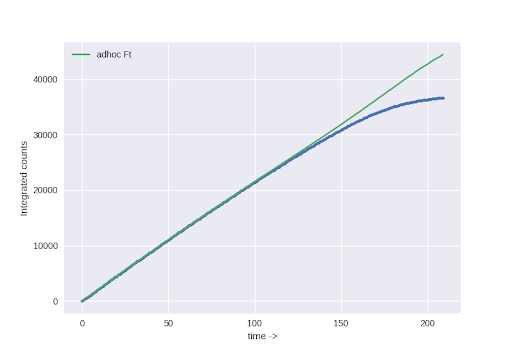
The HPF pipeline, cleans up the bias fluctuations in the “up-the-ramp” data, applies non-linearity correction, and cosmic-ray recovery to create a clean data cube. More details of these algorithms are provided in SPIE: 107092U Figure on the right shows a typical example of the up-the-ramp readout of a pixel, and the nonlinearity corrected line. Slope estimates of each pixel are used to generate a 2D slope (flux) image from the 3D “up-the-ramp” data. These slope images are stored in FITS files at the following location on TACC:
DATE/hpf/reduced/OBSID/Slope-YYYMMDDThhmmss_R01.fits
The Slope fits images have the following four extensions: 1. Flux (slope) image in units of e-/sec 2. Variance image which provides the pixel level variance of the flux estimate in the first extension. (unit: (e-/sec)^2) 3. Number of non-destructive reads used in the slope calculation of each pixel form the up-the-ramp data. 4. An array of average “up-the-ramp” curves of different region of interests. These one-dimensional summary of the increase in the counts during the ramp exposure is provided for diagnostic purpose. The mask defining those regions are provided on the TACC at /work/03946/hetdex/maverick/HPF_Processed/MasterCals/HPFmask_liberal_v5.fits
1D Extracted Spectra
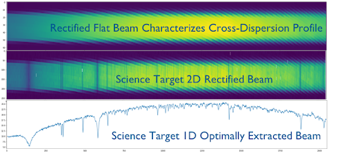
The HPF data reduction pipeline extracts each 2D slope image into a 1D spectrum as follows:
- The slope image is flat fielded using a scattered light flat that illuminates the entire detector area. This corrects achromatic pixel-to-pixel QE variations. It does not correct for the instrument response, nor for chromatic QE. To correct these effects, see the section below “Flat Fielding with Alpha Brights”
- Mask static bad pixels. This mask is provided in the ancillary data products folder on TACC.
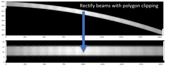
- Trace the beams and extract with an optimal extraction algorithm (e.g. Horne 1986). The cross-dispersion profile has been derived from Alpha Bright flats. Beams are rectified prior to extraction using the flux conserving polygon clipping algorithm from Smith et al. 2013
An instrumental drift corrected wavelength solution is provided in the last three extensions of the extracted spectrum. The instrumental drift is calculated by linear interpolation of the drift estimates from the nearest data containing LFC comb in cal fiber. The drift corrected wavelength solution is calculated at an order by order basis by interpolating the drift value to the flux weighted midpoints of each order. If the S/N of the flux rate curve during an exposure is less than 2, then the curve is averaged across the orders for a more stable solution. The chromatic flux weighted midpoint of each order matter only if one is doing precision RV on bright targets. The master wavelength solution itself is calculated by fitting the comb lines in the Laser Frequency comb data. The pixel level wavelength solution of each extracted pixel is stored like an image array in the same format as the flux arrays. The wavelengths are all provided in vacuum wavelengths (unit: Angstroms).
The final 1D optimally extracted spectra flux, variance, and wavelength solutions are stored in FITS files as 2D arrays with the following FITS extensions:
- Science fiber flux in units of (e-/sec)
- Sky fiber flux in units of (e-/sec)
- Calibration fiber flux in units of (e-/sec)
- Science fiber variance in units of (e-/sec)^2
- Sky fiber variance in units of (e-/sec)^2
- Calibration fiber variance in units of (e-/sec)^2
- Science fiber’s wavelength per pixel (Vacuum wavelength in Angstroms)
- Sky fiber’s wavelength per pixel (Vacuum wavelength in Angstroms)
- Calibration fiber’s wavelength per pixel (Vacuum wavelength in Angstroms)
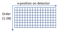
The x-axis of the 2D arrays correspond exactly to the x-axis on the detector and the y-axis correspond the the echelle order (1-28) starting from bluest on the top row to reddest on the bottom row. The array reads like a book (left-to-right and top-to-bottom) in order of increasing wavelength.
FITS header keywords added for 1D extractions
- Primary Extension
- E_VER - Extraction code version number.
- “vX.YZ”
- E_GIT - Extraction code current git commit
- Long string of letters and numbers for git commit to https://github.com/psuastro/HPFdrs
- RECTIF - Are rectified beams used for 1D extraction?
- Always true ”T”
- EXTRACT - Type of 1D extraction (“optimal” or “sum”)
- Always “optimal”
- CHECKSUM - HDU checksum
- DATASUM - data unit checksum
- Always “0” for primary extension
- E_VER - Extraction code version number.
- Extension 1 (or higher)
- XTENSION - Extension type added by astropy.io.fits. Always an image for the extraction code outputs.
- Always “IMAGE”
- BITPIX - Array data type added by astropy.io.fits. Always 32 bit floating point.
- Always “-32”
- NAXIS - Number of dimensions in array stored in fits extension. 2 for 1D extractions
- Always “2” for 1D extractions
- NAXIS1 - Number of pixels in dimension 1
- Always “2048” for HPF
- NAXIS2 - Number of pixels in dimension 2
- “28” for number of orders in HPF 1D extractions
- PCOUNT - Number of parameters. Added by astropy.io.fits.
- Always “0”
- GCOUNT - Number of groups. Added by astropy.io.fits.
- Always “1”
- EXTNAME - Type of data stored in this extension. Name of fiber and then name of datatype
- “Sci/Sky/Cal Flux/Variance” for extractions or rectified beams
- CTYPE1 - Units type for dimension 1 pixels.
- Always “X” *CTYPE2 - Unit type for dimension 2 pixels
- Always “Order”
- CHECKSUM - HDU checksum
- DATASUM - data unit checksum
- XTENSION - Extension type added by astropy.io.fits. Always an image for the extraction code outputs.
Flat fielding with Alpha Brights
This version of data release does not do a flat fielding in the 2D image before extraction using the continuum source Alpha Bright Cals taken everyday. However, before the extraction step, we do a zeroth order flat correction of quantum efficiency and gain differences the pixels using a median filtered scattered light flat. (Normalisation by the median filtered smooth image of the scattered light flat is to remove low frequency components in the scattered light pattern, which are not true pixel effects). This step does not correct for the high frequency instrumental response nor the chromatic QE of the detector pixels. Hence it is important to flat field the spectrum using alpha bright. Since HPF’s slit is rectangular and there is minimal wavelength overlap in extraction of pixels along the slit, to a good extent it suffices to flat field the extracted spectrum using the extracted alpha bright frames. Nightly cals taken routinely include alpha bright frames (Alpha Bright Cal: for Cal fiber) and (Alpha Bright FCU: for Sci and Sky fibers). If flat fielding is done using the extracted spectrum, it is important to use the same optimal extracted spectrum generated by the pipeline. For the data taken in the Shared Risk period (2018 May to July), the alpha brights taken in Sci and Sky fibers via FCU head, suffers from modal noise. Hence, one should be careful interpreting any continuum structures less than 1% after using Alpha Bright FCU flats. If available, we recommend using flats generated from A or B type standard stars. HPF detector has an epoxy void which is known to behave differently from frame to frame. It is recommended to be careful to interpret any features which falls along the edges of this void.
In future releases, we will be providing better flat corrected data for the user community.
![]()
Auxiliary Files
On the TACC cluster at the following directory
/work/03946/hetdex/maverick/HPF_Processed/MasterCals
we have kept the following auxiliary files which would be useful for the community:
- HPFmask_liberal_v5.fits
- Bad pixel mask
- HPF_NFlAT_20180203.fits
- Scattered light flat field
- HPF_DiagnosticRegionMask28Nov2017.npy
- An array with the regions used for the diagnostic average up-the-ramp curves stored in the 4th extension of the slope images.