Exposure times and Phase II information
This post contains some useful resources to prepare Phase II proposals / TSL submissions to observe with HPF.
Submitting HPF Phase IIs
The Phase II's for HPF are prepared using the common TSL files for HET. Let's dive right in and take a look at an example HPF TSL file.
Example HPF TSL file (Updated Aug 1st, 2020)
Below is an example TSL file to observe 3 sample stars, now using the dedicated HPF TSL keywords. Exposure times should be given in seconds which will then be converted by the RAs at HET to the closest number of reads (one read is 10.5s).
COMMON
   PROGRAM YYY20-3-XXX
   INSTRUMENT HPF
   SEEING 2.5
   SKYTRANS S
   EQUINOX 2000.0
   PMEPOCH 2015.0
   SKYBRIGHT_I 18
   SKYCALS N
   TELL N
   FLUX N
   SNWAVE 10000
TRACK_LIST
OBJECT        RA        DEC PMRA PMDEC IMAG JMAG EXP PRI NUMEXP VISITS HPFCOMPARISON SNGOAL SETUPMETHOD EXTRACALS
TARG1 12:34:56.7 12:34:56.7 -1.9  2.3  9.5  8.0  300   1 3      10     LFC           173    DirectACAM  1xcalLFCadj
TARG2 12:34:56.7 12:34:56.7 -1.2 -2.3  11.0 9.4  900   2 2      10     None          158    DirectACAM  1xcalLFCadj
TARG3 12:34:56.7 12:34:56.7  5.1  3.8  6.0  5.5  200   3 3      10     LFC           447    HPFACAM     1xcalLFCadj
- The maximum exposure time with the HPF LFC is 315s (LFC saturation)
- The maximum exposure time with HPF is 945s. Longer exposures will have to be split into shorter exposures, each of maximum length of 945s. This is set by the HPF Pipeline, not hardware.
- The minimum exposure time with HPF is 21s.
- Saturation happens at SNR~650 (see exposure calculator below) Do not go over this limit, as this will produce significant persistance on the HPF H2RG.
- When observing with HPF, using the following keywords is required:
-- HPFCOMPARISON: None / LFC, to indicate if you want the LFC on or off
-- SETUPMETHOD: DirectACAM/HPFACAM, to indicate if you want a direct setup or a regular setup (see further description below).
-- JMAG: J magnitude of the target.
-- SNGOAL: to indicate the estimated SNR of the observation. This is helpful for the Resident Astronomers to check the quality of the observation (e.g., on a cloudy night). Do note that this is per individual observation rather than for the full visit. The SNR will be evaluated at the wavelength denoted by the SNWAVE keyword. See the HPF Exposure Time Calculator below to estimate SNRs for different stars at 10000A. Generally we suggest putting the "Median" SNR from the HPF calculator here to account for seeing and pupil variations.
A few further points to keep in mind are:
Proper motions and current epoch
The HET TSL now takes in proper motions via the PMRA and PMDEC keywords. Therefore, the RA/DEC coordinates should be given in J2000 with the corresponding proper motions given using the PMRA/PMDEC keywords. The HET submission system will propogate the coordinates correctly to the current date of observations.
Using the HPF Laser Frequency Comb
The maximum exposure time for the HPF LFC through the HPF calibration fiber is 315s (30 reads), as otherwise there is a risk of the LFC comb lines saturating the HPF detector. The LFC should be used for the highest precision RV work. However, we recommend not using the LFC for faint sources, as it can contaminate the faint source spectrum. You can specify to use the LFC by using the HPFCOMPARISON keyword.
Acquisition modes
HPF has two acquisition modes. Currently, these modes are requested by use of the SETUPMETHOD keyword.
The two modes are:
1) Regular Setup (Imag < 11, SETUPMETHOD: HPFACAM): This mode uses the HPF CFB-bundle acqusition camera, and is available for science targets that are brighter than I-magnitude of 11. This mode uses requires the following steps:
- Center the star in the HPF CFB bundle camera
- Perform a deterministic offset to send the science target light through the HPF science fiber.
2) Direct Setup (Imag >11, SETUPMETHOD: DirectACAM): This mode is for stars that are too faint to be acquired with the HPF CFB-bundle acquisition camera, and instead makes use of the HET ACAM, which can slide in-and-out of the HET focal plane. This mode uses requires the following steps:
- Acquire a bright star using method #1 above to acquire a well defined centroid. Currently, it is up to the RAs to choose which star to define the centroid. They will try to find a close-by bright star to minimize overheads.
- Slide in the HET ACAM into the beam path to define acquire a well-defined offset fiducial.
- Slew to the science target with the HET ACAM still in the beam path.
- Center the target science target on the HET ACAM fiducial position.
- Perform a deterministic offset to send the science target light through the HPF science fiber.
Estimating HPF Exposure Times
This section contains a few useful resources for calculating HPF exposure times, including an online exposure time calculator and a Python function to estimate exposure times.
HPF Exposure time Calculator
The following calculator accounts for read noise from the different number of reads:
SNR and Exposure time plots
For the plots and functions below, please note:
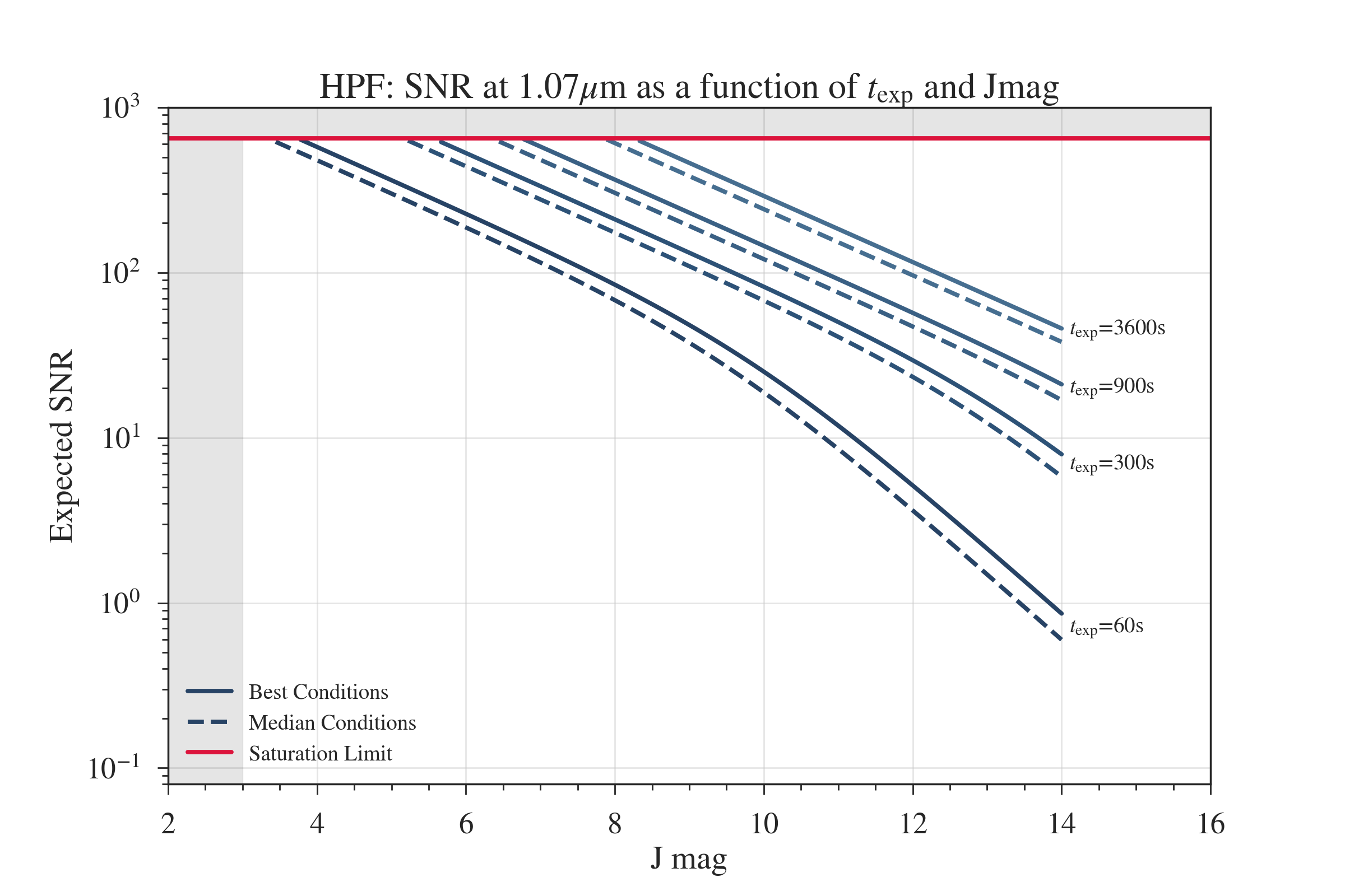
- SNR is defined as the SNR per 1D extracted pixel (which roughly corresponds to 10 pixels on the HPF echellograph), at 1.07micron. This corresponds to HPF Order 18 (starting counting at 0). This is the brightest cleanest order for an ~M4-dwarf in the HPF bandpass.
- The minimum allowable exposure time with HPF is 21s, and the brightest objects allowed are \(J = 3.0 \). Our recommended shortest exposure time is at least 60s, to get a better handle on the up-the-ramp slopes.
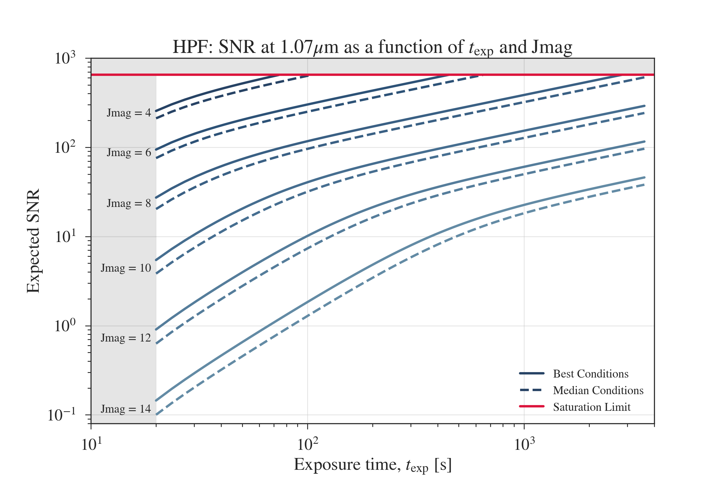
- 'Best conditions': observed during the peak of the HET track, and during good seeing conditions (between 1-1.5arcseconds at HET).
- 'Median Conditions': median observed SNR during HPF commissioning and engineering. We suggest to use this value for the SNGOAL keyword in the TSL to account for seeing effects and pupil illumination variations of the HET.
SNR including readout noise: SNR as a function of J-mag, with fixed exposure time curves
The plot below shows the expected HPF SNR as a function of J-mag. This plot accounts for readout noise effects.
SNR including readout noise: SNR as a function of exposure time, with fixed J-mag curves
The plot below shows the expected HPF SNR as a function of exposure time. This plot accounts for readout noise effects.
Exposure time as a function of J-mag for given SNRs
The graph below shows the required exposure time needed (green dashed curve) to achieve a Signal-to-Noise-Ratio (SNR) of 100 at 1.07microns (HPF Order #18) under best conditions, for a given star of J-magnitude \( m \). To begin with, we decided to use HPF Order 18---corresponding to 1.07micron---as that is the brightest cleanest order for early-mid M-dwarfs in the HPF bands. Orders 19 and 20 can be brighter (at the 5 - 10% level) but they have more telluric absorption. This plot does not account for readnoise.
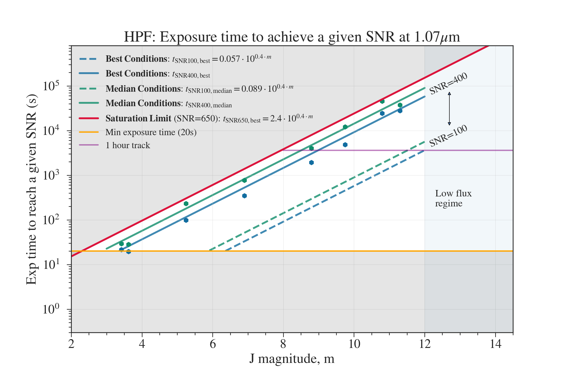
The approximate exposure time can be given by the following equation:
$$t_{\mathrm{exp}}(m,S) = 0.057 \cdot 10^{0.4 \cdot m} \cdot \left( \frac{SNR}{100} \right)^2,$$ where \( m \) is the J magnitude of the host star and \( SNR \) is the desired SNR. This formula is correct in the shot-noise limit. In the regime where read noise dominates (faint stars, and short exposuretimes), please use the exposure time calculator above, which accounts for readnoise.
A few notes on Saturation and Persistance on the HPF H2RG
- Saturation happens at roughly SNR = 650.
- We recommend to plan your observatios so that they are SNR<600 per exposure to minimize risk of persistance for you and other HPF observers.
- Saturation is defined as achieving 30,000 counts/pixel on the 2D echellogram on the H2RG, corresponding roughly to 300,000 counts/pixel in the 1D extracted spectrum.
Estimating exposure times in Python
A simple Python function to estimate exposure times is below. Please note, however, that this function does not account for readout noise. You can find further Python functions to make the plots in this article, and to calculate HPF exposure times and SNRs including read noise effects on GitHub here: https://github.com/gummiks/HPF-SNR-plots.
def t_exp(jmag,snr,verbose=True):
    """
    HPF exposure time in seconds to get a given SNR at 1.07micron.
    This function does not account for read noise.

    NOTES:
    See https://github.com/gummiks/HPF-SNR-plots for more accurate functions
    that include read noise.
    """
    assert jmag > 3.0
    assert snr < 650
    k, C = 0.40, 0.057
    t = C*10**(k*jmag)*((snr/100.)**2.)
    # Provide a warning if exposure time is too short
    if verbose and t < 21.:
        print("Warning. Exposure time < 21 s")
    return t
If you have any questions and/or suggestions for improvement, don't hesitate to send an email to gudmundur - at - psu.edu.